I love the idea of literate programming with R Markdown. Over the last 18 months, I’ve fallen away from daily R use, but I’ve been meaning to get back into writing with .Rmd. I recently scrapped my old blog and decided to start a fresh one, so thought this would be the time to get back into the habit.

I’m still blogging with Jekyll and GitHub Pages, but this time around I’m aiming for a workflow that at least feels like it has less dependencies (maybe it won’t, but I’ll probably learn some things along the way to failure). Previously, I wrote all my posts in .Rmd, compiled them with knitr and rmarkdown via servr::jekyll(), and pushed to my GitHub remote from there. This time, I’ve moved all the compilation into a self-rolled script so everything can be built or served with a Makefile.

If you’re interested in how this is done, check out the repo here and pay special attention to ./Makefile and ./build.R. Instead of jekyll serve, you can use make serve to compile the .Rmd into _posts/ and then automatically serve the site from there.

(Edit: July 10) Now all of the R Markdown compilation is kicked off by a ridiculously simple Jekyll :pre_render hook:

Jekyll:Hooks.register :site, :pre_render do |doc, payload|
    `Rscript build.R`
end

I just have to run jekyll serve like usual. 🥳

For posterity (and so I can review all the CSS), here’s some placeholder text demoing what works:

R Markdown

This is an R Markdown document. Markdown is a simple formatting syntax for authoring HTML, PDF, and MS Word documents. For more details on using R Markdown see http://rmarkdown.rstudio.com.

You can embed an R code chunk like this:

summary(cars)

##      speed           dist
##  Min.   : 4.0   Min.   :  2.00
##  1st Qu.:12.0   1st Qu.: 26.00
##  Median :15.0   Median : 36.00
##  Mean   :15.4   Mean   : 42.98
##  3rd Qu.:19.0   3rd Qu.: 56.00
##  Max.   :25.0   Max.   :120.00

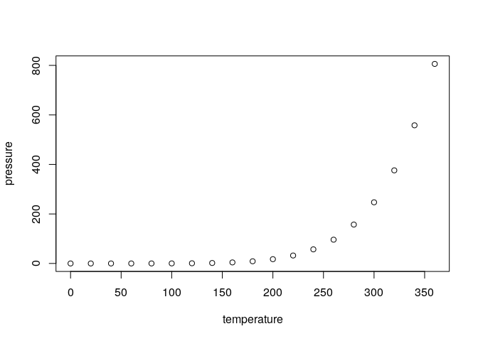
Including Plots

You can also embed plots, for example:

Other Languages

Code chunks in other languages can also be embedded. Create a fenced code block that begins with a declaration like this:

```{python}
import pandas as pd

df = pd.DataFrame({"a": [1, 2, 3], "b": [4, 5, 6]})
df
```

The block will be executed and run like R code chunks, for example:

import pandas as pd

df = pd.DataFrame({"a": [1, 2, 3], "b": [4, 5, 6]})
df

##    a  b
## 0  1  4
## 1  2  5
## 2  3  6

Objects in other languages can be accessed in subsequent chunks, as with R chunks, like:

import torch

x = torch.tensor(df.values, dtype=torch.long)
x.size()

## torch.Size([3, 2])

Many objects are also easy to share back and forth across Python and R environments using the py object exported by reticulate like:

str(reticulate::py$df)

## 'data.frame':    3 obs. of  2 variables:
##  $ a: num  1 2 3
##  $ b: num  4 5 6
##  - attr(*, "pandas.index")=RangeIndex(start=0, stop=3, step=1)

\(\LaTeX\)

It is also possible to include both inline and fenced math using the $$ syntax. For example, \(f(x) = tan^{-1}(x)\), or: